A generic approach for training probabilistic machine learning models

Nicolas Arroyo nicolas.arroyo.duran@gmail.com

Introduction

Neural networks are universal function approximators. Which means that having enough hidden neurons a neural network can be used to approximate any continuous function. Real world data, however, often has noise that in some cases makes producing a single deterministic value prediction insufficient. Take for example the dataset in Fig. 1a, it shows the relation between the departure delay and the arrival delay for flights out of JFK International Airport over a period of one year (Subset of 2015 Flight Delays and Cancellations).

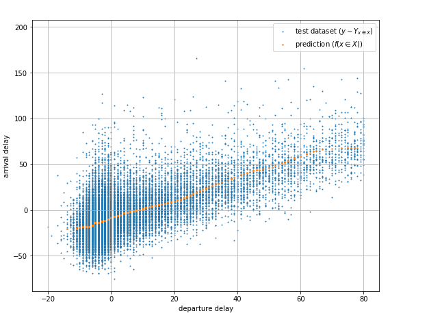Fig. 1a Departure to arrival delays from JFK

Fig. 1a also shows the prediction of a fully trained neural network that does a good job of approximating the mean value and does provide information about the trend of the dataset. However, it does not help answer questions like given a departure delay, what is the maximum expected arrival in X% of the flights? or given a departure delay, what is the probability that the arrival delay will be longer than Y? or even more interesting, write a model that samples arrival delay values for given departure delays with the same distribution as the real thing.

There are methods to solve this problem, for example, assuming the model in Fig 1a estimates the mean, the standard deviation for the entire data set can be calculated and with those parameters you can produce the expected normal distribution. And if the variance is not constant, that is if the variance changes across the input space, you could use Logistic Regression with Maximum Likelihood Estimation which in a nutshell trains a model that predicts the parameters for a specific distribution function (for example the mean and the standard deviation of the normal or gaussian distribution) at a given input. The problem is that it relies on beforehand knowledge of the dataset distribution, which might be difficult in some cases or too irregular to match a known distribution.

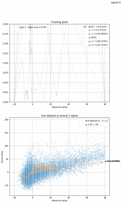
In the case of the departure to arrival delays dataset, we can observe from the plot that the distribution appears to be similar to the normal distribution, so it makes sense to build a Maximum Likelihood Estimation model trying to calculate the parameters of a normal distribution. Fig 1b shows a plot of a fully trained model showing the mean, the mean plus/minus the standard deviation and the mean plus/minus twice the standard deviation. The error of this model is of 2.48% which is quite good. However, the dataset's distribution is not perfectly normal, you can see that the upper tail is slightly longer than the lower tail in addition to other imperfections, which is why the accuracy is not better.

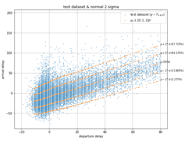Fig. 1b Departure to arrival delays from JFK and probabilistic model

This article presents a generic approach to training probabilistic machine learning models that will produce distributions that adapt to the real data with any distribution it may have, even branching distributions or distributions that change form across the input space.

The method

Given that the function producing the data has a specific distribution Y at input x ∈ X ¹ we can define the target function, or the function we actually want to approximate, as y ∼ Yₓ. We want to create an algorithm capable of sampling an arbitrary number of data points from Yₓ ² for any given x ∈ X.

To do this we introduce a secondary input z that can be sampled from a uniformly distributed space Z ³ by the algorithm and fed to a deterministic function f such that P(Z < z) = P(Yₓ <= f(x, z)).

Or put another way, we want a deterministic function that for any given input x, maps a random (but uniform) variable Z to a dependent random variable Yₓ.

Model

The proposed model to approximate Yₓ is an ordinary feed forward neural network that in addition to an input x takes an input z that can be sampled from Z.

Overview

At every point x ∈ X we want our model f(x, z ∼ Z) to approximate the Yₓ distribution to an arbitrary precision. Let's picture f(x, z ∼ Z) and Yₓ as 2-dimensional (in the case where X and Z are both 1-dimensional) pieces of fabric, they can stretch and shrink in different measures at different regions, decreasing or increasing their densities respectively. We want a mechanism that stretches and shrinks f(x, z ∼ Z) in a way that matches the shrinks and stretches in Yₓ.

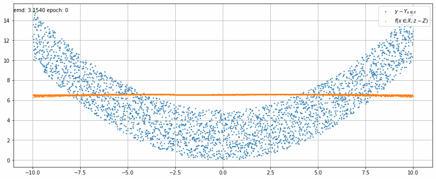Fig 2 An animation of the training to match x² with added uniform noise.

In Fig 2 we can see how the trained model output stretches and shrinks little by little on each epoch until it matches target function.

Going on with the stretching and shrinking piece of fabric analogy, we want to put "pins" into an overlaying fabric (our model) so that we can superimpose it over the underlying fabric (the target data set) that we are trying to match. We will put these pins into fixed points in the overlaying fabric but we will move them to different places of the underlying fabric as we train the model. At first we will pin them to random places on the underlying fabric. As we observe the position of the pins on the underlying fabric relative to the overlaying fabric we will move them slightly upwards or downwards to improve the overlaying fabric's match on the underlying fabric. Every pin will affect its surroundings in the fabric proportionally to distance from the pin.

We'll start by putting 1 pin at a fixed position in any given longitude of the overlaying fabric and at the midpoint latitude across the fabric's height. We'll then make many observations in the underlying fabric at the same longitude, that is we will randomly pick several locations at the vertical line that goes through the selected pin location.

For every observed point, we'll move the pin position on the underlying fabric (keeping the same fixed position on the overlaying fabric) a small predefined distance downwards if the observed point is below its current position, and we'll move it upwards if it is above it. This means that if there are more observed points above the pin's position in the underlying fabric the total movement will be upwards and vice versa if there are more observed points below it. If we repeat this process enough times, the pin's position in the underlying fabric will settle in a place that divides the observed points by half, that is the same amount of observed points are above it as below it.

Why do we move the pin a predefined distance up or down instead of a distance proportional to the observed point? The reason is that we are not interested in matching the observed point. Since the target dataset is stochastic, matching a random observation is pointless. The interesting information we get from the observed points is whether or not the pin divides them by half (or by another specific ratio)

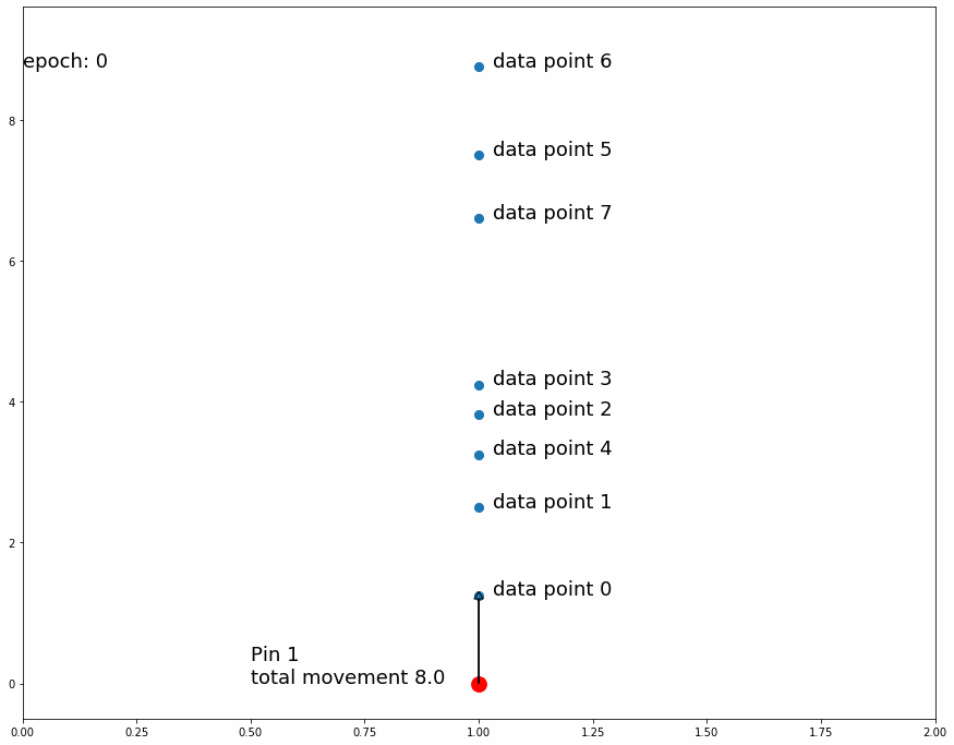Fig 3 Moving 1 pin towards observed points until it settles.

Fig 3 shows how the pin comes to a stable position dividing all data points in half because the amount of movement for every observation is equal for data points above and data points below. If the predefined distance of movement for observations above is different from the predefined distance of movement for observations below then the pin would settle in a position dividing the data points by a different ratio (different than half). For example, let's try having 2 pins instead of 1, the first one will move 1 distance for observations above it and 0.5 distance for observations below, the second one will do the opposite. After enough iterations the first one should settle at a position that divides the data points by 1/3 above and 2/3 below while the second pin will divide by 2/3 above and 1/3 below. This means we'll have 1/3 above the first pin, 1/3 between both pins and 1/3 below the second pin like Fig 4 shows.

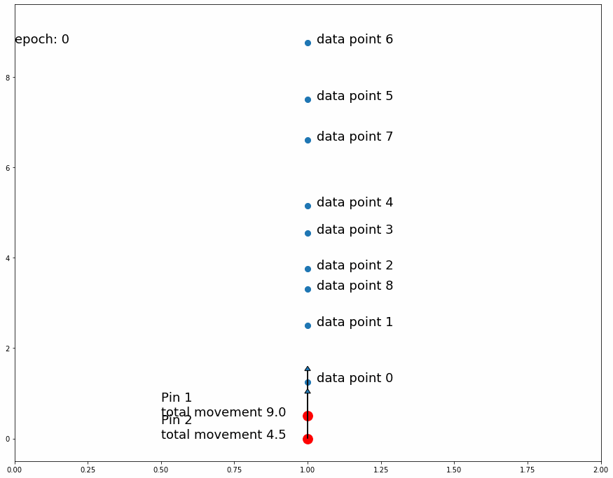Fig 4 Moving 2 pins towards observed points until they settle.

If a pin divides the observed data points in 2 groups of sizes a and b and after training its fixed position settles in the underlying fabric in the a/(a+b) latitude from the top, we have a single point mapping between the 2 fabrics, that is at this longitude the densities above and below the pin are equal in both pieces of fabric. We can extrapolate this concept and use as many pins as we want in order to create a finer mapping between the 2 pieces of fabric.

Definitions

We'll start by selecting a fixed set of points in Z of size S that we will call z-samples. We can define this set as:

<<< Insert image 1 >>>

The predictive model will be defined as:

<<< Insert image 2 >>>

Here x will be any input tuple from the input domain, z will be a sample from uniform random variable Z and θ is the internal state of the model, or the weight matrix.

Then we define the prediction error for any input x for a specific z ∈ Z as:

<<< Insert image 3 >>>

That is, the difference between the real data cumulative probability distribution and the predicted cumulative probability distribution.

Now we can define our training goals as:

Goal 1

<<< Insert image 4 >>>

In other words, we want that for every z' in zₛₐₘₚₗₑₛ and across the entire X input space the absolute error |E(z')| is minimized. This first goal gives us an approximate discrete finite mapping between the z-samples set and Yₓ. Even if it doesn't say anything about all the points ẑ in Z that are not in zₛₐₘₚₗₑₛ.

Goal 2

<<< Insert image 5 >>>

This second goal gives us that for any given x in X, f is a monotonically increasing function in Z.

Both of these goals will be tested empirically during the testing step of the training algorithm.

Model accuracy

For any point z ∼ Z and with z' and z'' being the z-samples that are immediately smaller and greater respectively, and assuming Goal 2 is met we have:

<<< Insert image 6 >>>

and replacing the prediction error we have:

<<< Insert image 7 >>>

And if we substract P(Z <= z) from every term we have:

<<< Insert image 8 >>>

What this means is that for any point z ∼ Z the prediction error error E(z) is lower bounded by P(Z <= z') - P(Z <= z) + E(z') and upper bounded by P(Z <= z'') - P(Z <= z) + E(z'').

Assuming Goal 1 is met we know that E(z') and E(z'') are small numbers which leaves P(Z <= z') - P(Z <= z) and P(Z <= z'') - P(Z <= z) as the dominant factors. The distance between any z and its neighboring z-samples can be minimized by increasing the number of z-samples or S. In other words the maximum error of f can be arbitrarily minimized by a sufficiently large S.

Calculating the movement scalars

Having defined our goals and what will they buy us, we move to show how we will achieve Goal 1. For simplicity we will use a z-samples set that is evenly distributed in Z, that is: {z[0], z[1], ... , z[S-1]} ∈ Z s.t. z[0] < z[1], ... , < z[S] ∧ P(z[0] < Z < z[1]) = P(z[1] < Z < z[2]) = ... = P(z[s-1] < Z < z[s]).

For any given x in X and any z' in zₛₐₘₚₗₑₛ we want f to satisfy P(Yₓ <= f(x, z')) = P(Z <= z'). For this purpose we'll assume that we count with a sufficiently representative set of samples in Yₓ or yₜᵣₐᵢₙ ∼ Yₓ.

For a given x ∈ X and having z' as the midpoint in Z (i.e. z' ∈ Z s.t. Pr(z' <= Z) = 0.5) we could simply train f to change the value of f(x, z') a constant movement number M greater for every training example y ∈ yₜᵣₐᵢₙ that was greater than f(x, z') itself and the same constant number smaller for every training example that was smaller (remember the 2 pieces of fabric and the pins analogy). This would cause after enough iterations for the value of f(x,z') to settle in a position that divides in half all training examples when the total movement equals 0.

If instead of being Z's midpoint P(Z <= z') ≠ 0.5 then the constant numbers of movement for greater and smaller samples have to be different.

Let's say that a is the distance between z' and the smallest number in Z or Zₘᵢₙ, and b the distance between z' and Zₘₐₓ.

<<< Insert image 9 >>>

Since a represents the amount of training examples we hope to find smaller than z' and b the amount of training examples greater than z' we need 2 scalars α and β to satisfy the following equations:

<<< Insert image 10 >>>

These movement scalars will be the multipliers to be used with the constant movement M on every observed point smaller and greater than z' respectively. This first equation assures that the total movement when z' is situated at Zₘᵢₙ + a or Zₘₐₓ - b will be 0.

<<< Insert image 11 >>>

This second equation normalizes the scalars so that the total movement for all z in zₛₐₘₚₗₑₛ have the same total movement.

Which gives us:

<<< Insert image 12 >>>

This logic however, breaks at the edges, that is when a z-sample is equal to Zₘᵢₙ or Zₘₐₓ. At these values either a or b is 0 and if either of them is 0 then one of α or β is undefined.

As a or b approach 0 α or β tend to infinity, one might be tempted to replace this with a large number, but that would not be practical because a large distance multiplier would dominate the training and minimize the movement of other zₛₐₘₚₗₑₛ.

Also as one of α or β tend to infinity the other one becomes a small number that is also impractical but for a different reason. The zₛₐₘₚₗₑₛ at the edges are supposed to map to the edges of Yₓ and any quantity of movement into the opposite direction will result in Zₘᵢₙ or Zₘₐₓ mapping to a greater or smaller point in Yₓ respectively. For this reason the α and β for the zₛₐₘₚₗₑₛ at the edges (i.e. z[0] and z[S]) will be assigned a value of 0 for the one that pushes inward and a predefined hyperparameter C ∈ [0, 1] that can be adjusted to the model.

Training the model

In order to train the neural network the z-samples, the set size S is chosen depending on the desired accuracy and compute available. Having decided that, Z must be defined. That is, the number of dimensions and its range must be chosen. Given Z and the training level we can create the z-samples set.

For example if Z is 1-dimensional with range defined as [10.0, 20.0] and S = 9, we have that the z-sample set is {z₀ (10.0), z₁ (11.25), z₂ (12.5), z₃ (13.75), z₄ (15.0), z₅ (16.25), z₆ (17.5), z₇ (18.75), z₈ (20.0)}.

First we select a batch of data from the training data with size n, for every data point in the batch, we evaluate the current model on every z-sample. This gives us the prediction matrix:

<<< Insert image 13 >>>

For every data point (xᵢ, yᵢ) in the batch, we take the output value yᵢ and compare it with every value of its corresponding row in the prediction matrix (i.e. [f(xᵢ, z₀), f(xᵢ, z₁), ..., f(xᵢ, z₈)]). After determining if yᵢ is greater or smaller than each predicted value, we produce 2 values for every element in the matrix:

Movement scalar

The scalar will be α[z-sample] if yᵢ is smaller than the prediction and β[z-sample] if yᵢ is greater.

<<< Insert image 14 >>>

Target value

The target value is the prediction itself plus the preselected movement constant M multiplied by -1 if yᵢ is smaller than the prediction and 1 if yᵢ is greater. You can think of target values as the "where we want the prediction to be" value.

<<< Insert image 15 >>>

After calculating these 2 values we are ready to assemble the matrix to be used during backpropagation.

<<< Insert image 16 >>>

We pass the prediction matrix results in a addition to this matrix to a Weighted Mean Squared Error loss function (WMSE). The loss function will look like this:

<<< Insert image 17 >>>

Testing the model

The Mean Squared Error (MSE) loss function works to train the model using backpropagation and target values, but testing the model requires a different approach. Since both f(x, Z) and Yₓ are random variables, measuring the differences between their samplings is pointless. Because of this, the success of the model will be measured in 2 ways:

Earth Movers Distance (EMD)

In statistics, the earth mover's distance (EMD) is a measure of the distance between two probability distributions over a region D. In mathematics, this is known as the Wasserstein metric. Informally, if the distributions are interpreted as two different ways of piling up a certain amount of dirt over the region D, the EMD is the minimum cost of turning one pile into the other; where the cost is assumed to be amount of dirt moved times the distance by which it is moved. wikipedia.org

Using EMD we can obtain an indicator of how similar Yₓ and f(x, Z) are. It can be calculated by comparing every x, y data point in the test data and prediction data sets and finding way to transform one into the other that requires the smallest total movement. What the EMD number tells us is the average amount of distance to transform every point in the predictions data set to the test data set.

On the example below you can see that the mean EMD is ~3.9 on a data set with a thickness of roughly 100. Because of the random nature of the data sets the EMD cannot be used as a literal error indicator, but it can be used as a progress indicator, that is to tell if the model improves with training.

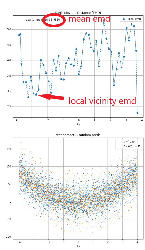Fig 5 EMD testing.

Testing the training goals

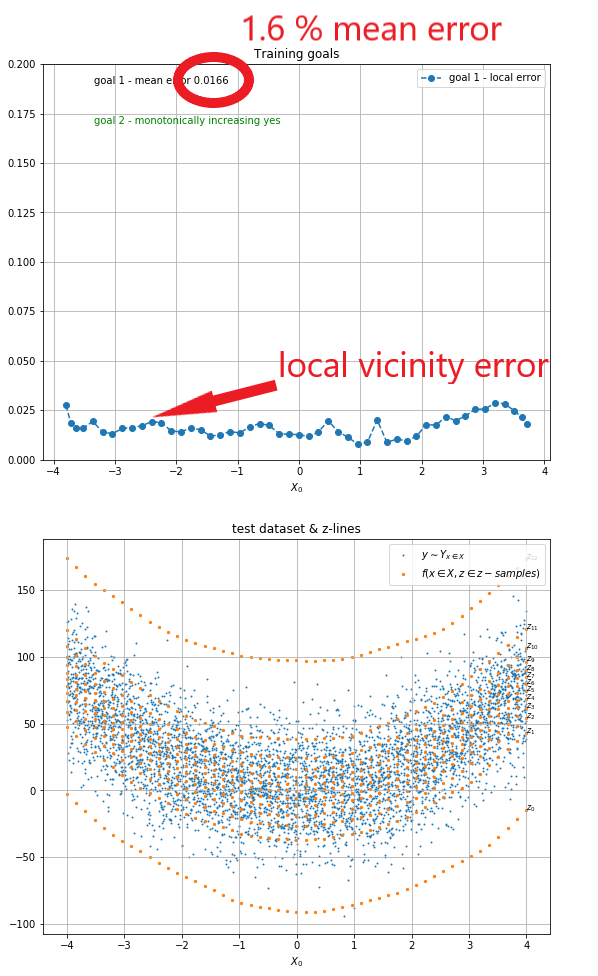
Training goal 1

Ideally to test Goal 1 (i.e. ∀ x ∈ X ∧ ∀ z' ∈ zₛₐₘₚₗₑₛ: arg min |E(z')|) we would evaluate f for a given x and on every z-sample and then compare it to an arbitrary number of test data points having the same x. We would then proceed to count for every z-sample the number of test data points smaller than it. With a vector of smaller than counts (i.e. P(Yₓ <= f(x, z'))) we could proceed to compare it with the canonical counts for every z-sample (i.e. P(Z <= z')) and measure the error. However in real life data sets this is not possible. Real life data sets will not likely have an arbitrary number of data points having the same x (they will unlikely even have 2 data points with the same x) which means that we need to use a vicinity in x (values X that are close to an x) to test the goal.

We start by creating an ordering (an array of indices) O = {o₀, o₁, ..., o[m]} that sorts all the elements in Xₜₑₛₜ (the x inputs in the test data set). Then we select a substring of the array O' = {oᵢ, oᵢ₊₁, ..., oⱼ}.

Now we can evaluate f for every x[o'] ∣ o' ∈ O' on every z-sample which gives us the matrix:

<<< Insert image 18 >>>

We then proceed to compare each row with the outputs y[o'] ∣ o' ∈ O'

<<< Insert image 19 >>>

and create smaller than counts (i.e. P(Yₓ <= f(x, z))) which we can then compare with the canonical counts for every z-sample (i.e. P(Z <= z)) to measure the error in the selected substring.

We will create a number of such substrings and call each error the local vicinity error located at the central element of the substring.

On the example below you can see that the goal 1 mean error is ~1.6%, this can be used as an error indicator for the model.

Fig 6 Training goal 1 testing.

Training goal 2

In order to test Goal 2 ∀ x ∈ X ∧ ∀ z₀, z₁ ∈ Z s.t. z₀ < z₁: f(x, z₀) < f(x, z₁) we select some random points in X and a set of random points in Z, we run them in our model and get result matrix:

<<< Insert image 20 >>>

From here it is trivial to check that each row is monotonically increasing. To increase the quality of the check we can increment the sizes of the test point set in X and the test point set in Z.

Back to delays

Now we can go back to the departure delays to arrival delays dataset, below you can see the MLE approach (Fig 7a) and the approach introduced in this article (Fig7b) side by side. As we saw before the MLE approach fails to capture the small imperfections obtaining a goal 1 error of 2.48% while the generic approach does a much better job with a 0.018% goal 1 error.

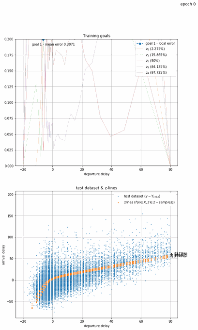Fig 7a Probabilistic model MLE approach.	Fig 7b Generic approach.

Experiments

The following are various experiments done on different datasets.

x² plus gaussian noise

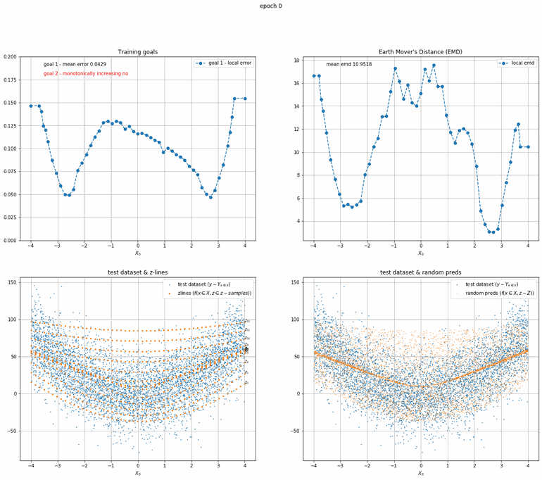
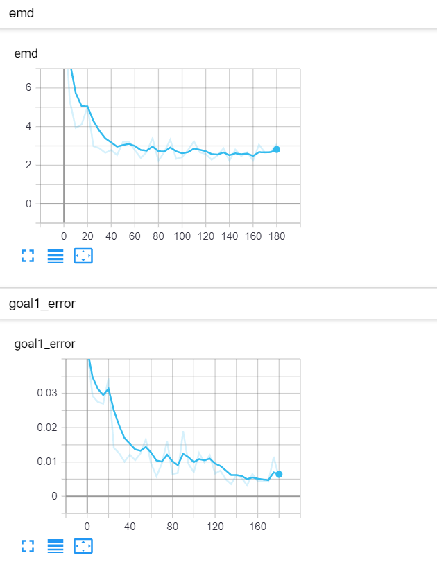
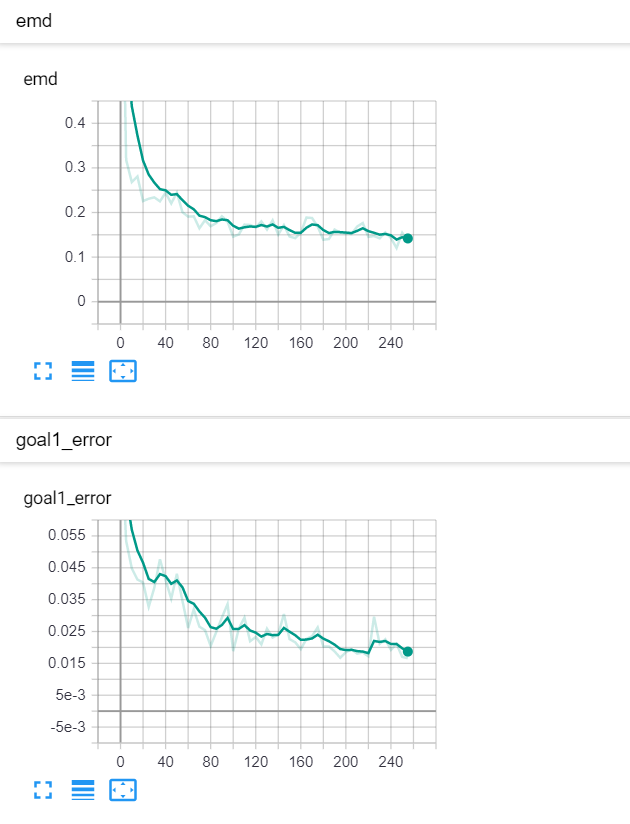
Let's start with a simple example. The function x² with added gaussian noise. On the left panel you can see the training evolving over the course of 180 epochs. On the top left corner of this panel you can see the goal 1 error localized over X, at the end of the training you can see that the highest local error is around 2% and the global error is around 0.5%. On the top right corner of the same panel you can see the local Earth Mover's Distance (EMD). On the bottom left corner you can see a plot of the original test dataset (in blue) and the z-lines (in orange), you can see how they progressively conform to the test data. On the bottom right you can see a plot of the original test dataset (in blue) and random predictions (with z ∼ Z), you can see as the predicted results progressively represent the test data.

On the right panel, you can see a plot of the global goal 1 error (above) and global EMD values (below) as they change over the course of the training.

Fig 8 Training model to match x² plus gaussian.

a x³ + bx² + cx + d plus truncated gaussian noise

This one is a bit more complicated. An order 3 polynomial with added truncated gaussian noise (that is a normal distribution clipped at specific points).

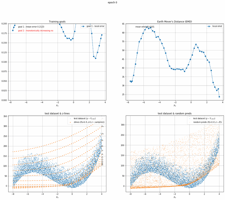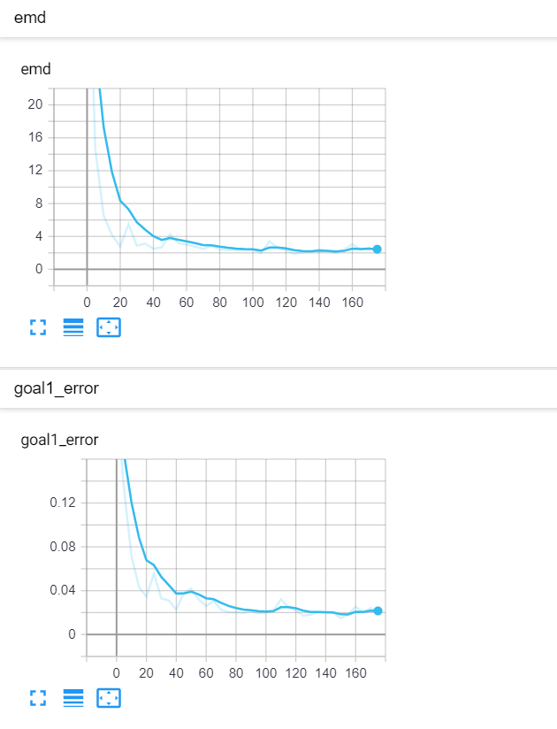Fig 9 Training model to match x³ + bx² + cx + d plus truncated gaussian.

Double sin(x) plus gaussian noise multiplied by sin(x)

This one is quite more interesting. 2 mirroring sin(x) functions with gaussian noise scaled by sin(x) itself.

<<< Insert image 21 >>>

Notice how the model succeeds to represent the areas in the middle with lower densities.

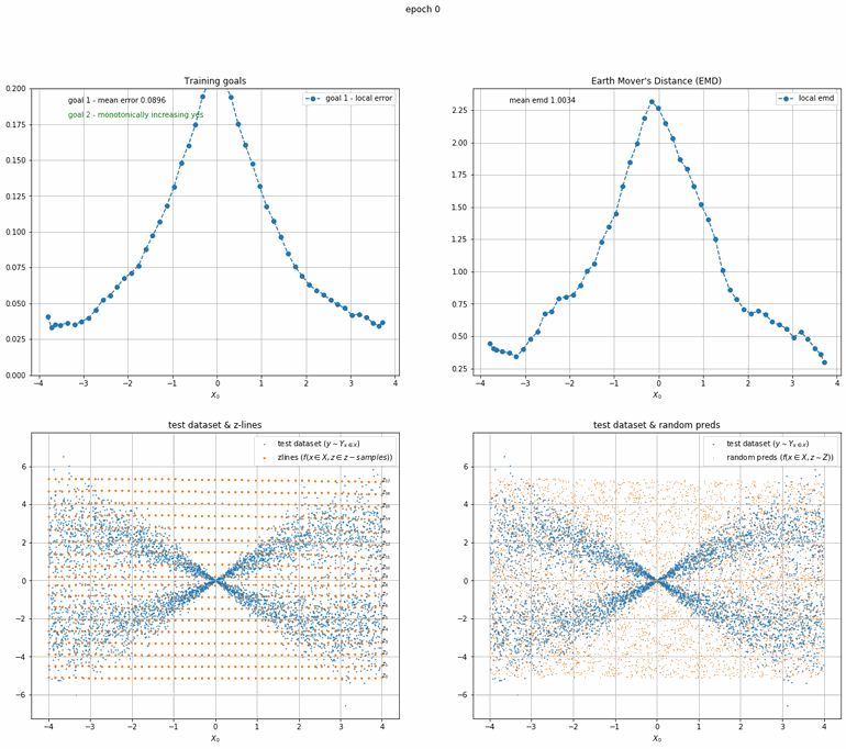Fig 10 Training model to match double sin(x) with added gaussian times sin(x).

Branching function plus gaussian noise

This one experiments with branching paths. It starts with simple gaussian noise around 0, then starts splitting it with equal probabilities over the course of various segments.

<<< Insert image 22 >>>

Despite the distribution not being continuous, the model does a reasonably good job of approximating it.

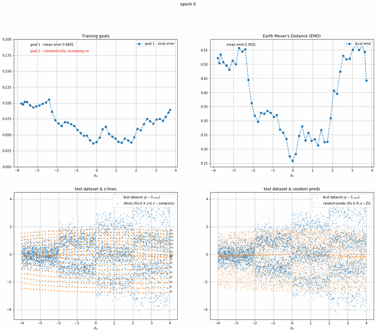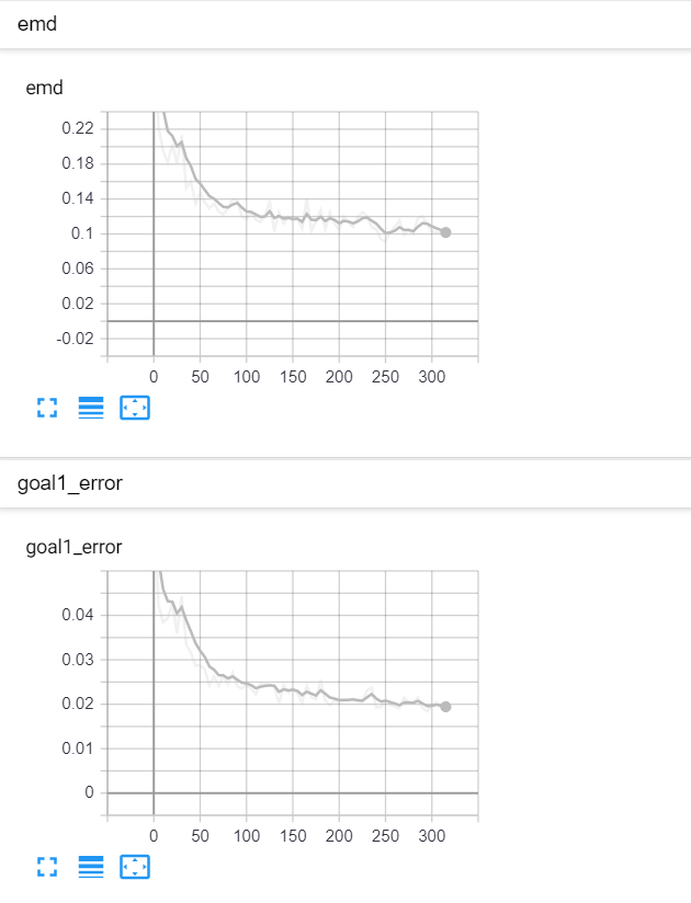Fig 11 Training model to match branching function plus gaussian.

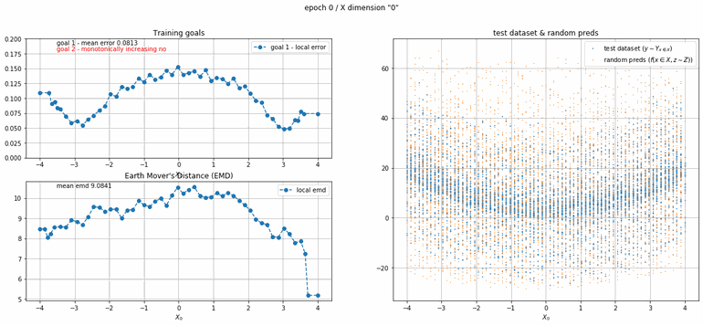
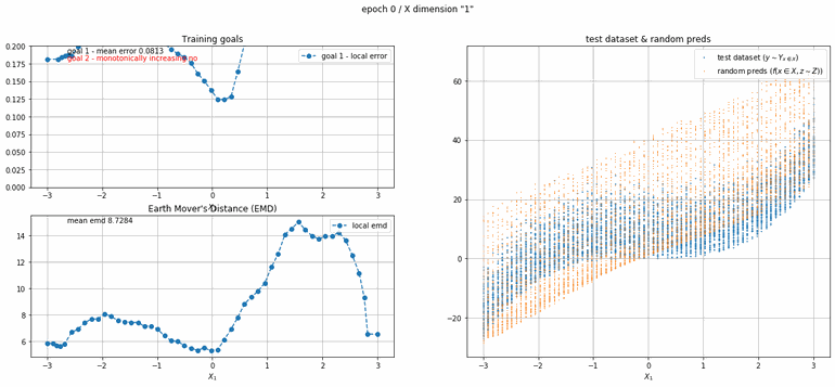
(x₀)² + (x₁)³ plus absolute gaussian noise

The next example has 2 dimensions of input. X₀ (the first dimension) is x² and X₁ (the second dimension) is x³ with added absolute gaussian noise. The display is slightly different, for the sake of space the z-lines plot is omitted. As you can see there is a panel per dimension and as always an additional panel for goal 1 error and EMD error histories.

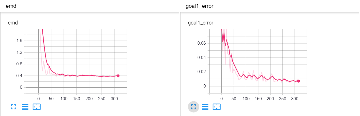Fig 12 Training model to match (x₀)² + (x₁)³ plus absolute gaussian.

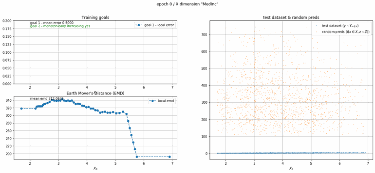
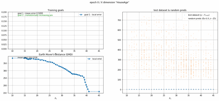
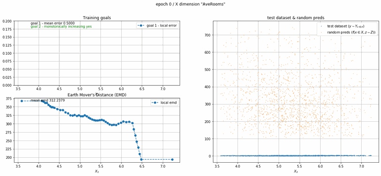
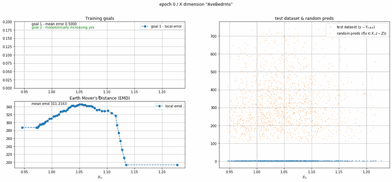
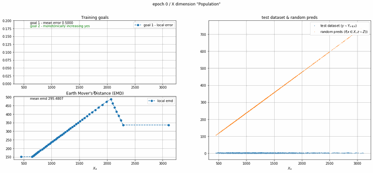
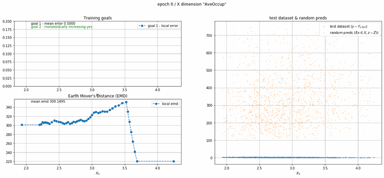
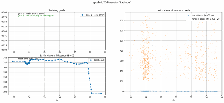
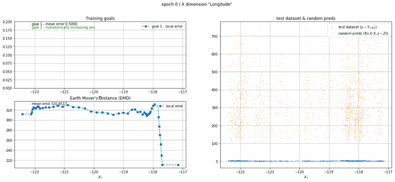
California housing dataset

This experiment uses real data instead of generated one which proves the model's effectivity on real data. It is the classic California housing dataset. It has information from the 1990 California census with 8 input dimensions (Median Income, House Age, etc ...). Below you can see the plots of each dimension.

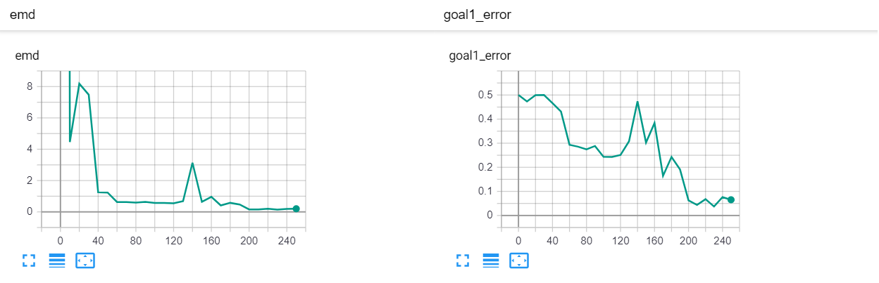Fig 13 Training model to match the California housing dataset.

Conclusion

The method presented allows to approximate the distributions of stochastic data sets to an arbitrary precision. The model is simple, fast to train and can be implemented with a vanilla feedforward neural network. Its ability to approximate any distribution across an input space makes it a valuable tool for any task that requires prediction.

References